Basic Concepts of Options

In our study of derivative pricing, we have so far examined forwards and futures, which constitute noncontingent claims. These contracts require both the writer and the holder to filfil their obligations to execute the contract at the expiration date. In this chapter, let us shift our focus to another crucial aspect of derivative markets: options. Options are contingent claims that offer a buyer the right, but not the obligation, to buy or sell an underlying asset at a predetermined price within a specified time frame. The buyer acquires the contingent claim by paying a premium to the contract. This unique characteristic of options makes them a valuable instrument for investors seeking strategic opportunities and risk management solutions in financial markets.

There are two primary types of options, namely, a call option and a put option. A call option gives the holder the right, but not the obligation, to buy an underlying asset at a predetermined price, known as the strike price, within a specified period. On the other hand, a put option grants the holder the right, but not the obligation, to sell an underlying asset at the strike price within a specified timeframe.

A key aspect of options theory is the concept of option premiums, their properties, and how their dynamics are modeled. Option premiums are influenced by various factors, including the current market price of the underlying asset, the time remaining until the option expiration, and market volatility. Factors such as interest rates and dividend payments may also affect option premiums. Understanding these factors is essential for traders as they evaluate potential option trades and assess the risk-reward profile of their strategies. Moreover, understanding option pricing mechanics allows investors to make informed decisions and effectively manage their portfolios in dynamic market environments.

In this chapter, we discuss some fundamental properties of option premiums. In Section «Click Here», we begin with an overview of the types of options, including call and put options, as well as the distinctions between American and European options. We also introduce the concepts of option payoffs and gains, providing the relationship between option payoffs and underlying asset prices. An option price comprises intrinsic value and time value. We discuss these two components of option pricing and provide formulas for various cases. Several option premium bounds are examined in Section «Click Here» for both European and American options under the no-arbitrage market condition. We also derive some important properties of option premiums that include the derivation and application of an important relation between the put and call premiums with same strike price and the underlying asset, known as put-call parity. The chapter concludes with key results on the relationship between premiums and strike prices, as well as the convexity property of option premiums.

Basic Terminology

An option contract involves two parties, the party initiating the contract is the writer or the seller of the option contract, while the counter party is the holder or the buyer.

Depending on the trade set in the contract, options can be categorized into two types:

Call Option: These options grant the holder the right but not the obligation to buy the underlying asset for a specified strike price by (or within) a predetermined time .
Put Option: These options grant the holder the right but not the obligation to sell the underlying asset for a specified strike price by (or within) a predetermined time.

To acquire the contingent position in the contract, the holder must pay a token amount upfront to the writer at the contract's acceptance time. This token amount is known as the premium or price of the option.

Note:

The price of an option ( i.e. the premium) should not be confused with the future or forward) price in a future (or forward) contract. A future price in a future contract is equivalent to the strike price in an option. Whereas the price of an option (often referred to as option price) is the amount paid by the holder to the writer in order to gain only the right but not the obligation to exercise the option contract ( i.e. the contingent position in the contract).

Remark:

The following is the list of all the basic parameters needed to define an option:

Contract issue time, generally taken as \(t=0\);
Expiration or maturity (date or time or both), denoted by \(t=T\);
Strike price or exercise price, denoted by \(K\);
Contract size, also called a lot size, which is the number of units of the underlying assets exercised in a contract; and
Option premium, denoted by \(X\) in general. When it comes to call option premium, we use the notation C and for the put option premium, we use P.

An option (a call or a put option) can further be categorized into two types depending on the time of execution of the contract. These are the American option and the European option.

American Option: In an American option, the contract can be exercised at any time up to the expiration time.

European Option: In a European option, the contract is allowed to be exercised only on the expiration time.

Note:

Before 2010, stock options in India were American, while index options were European. After 2010, all options in India became European.

The underlying asset of an option can include stocks, commodities, or foreign currencies, which are settled by physical delivery. However, there are also underlying assets that cannot be physically delivered at expiration, such as stock indices (like Nifty and Sensex) and interest rates. In these cases, settlements are made in cash by paying the difference between the strike price and the spot price.

Defining Parameters

Let \(S(t)\) (also denoted by \(S_t\)) be the spot market price of the underlying asset at any time \(t\) and \(K\) be the strike price of the option. Let the period of the option be \([0,T]\), where \(T\) is the expiration time or maturity. We proceed to find the payoff of an option at maturity \(T\).

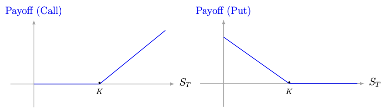
Observe first that, since the holder of an option has no obligation to exercise the option, the holder will exercise it if and only if there is a positive return. This means that

the holder of a call option will exercise it if and only if \(K < S_T\);
the holder of a put option will exercise it if and only if \(K > S_T\) (for European options).

Payoff and Gain

We begin by defining the payoff.

Definition:

[Payoff]

A call option is said to be

in-the-money if \(K < S_t\);
at-the-money if \(K=S_t\); and
out-of-the-money if \(K > S_t\),

at any time \(t\in [0,T]\). The payoff of a call option at the expiration \(T\) is defined as

\[ C_T =\left\{\begin{array}{ll} \max\big(0,S_T-K\big),&\text{ for buyer (long position)}\\ \min\big(0,K-S_T\big),&\text{ for seller (short position)} \end{array}\right. \]

A put option is said to be

in-the-money if \(K>S_t\);
at-the-money if \(K=S_t\); and
out-of-the-money if \(K < S_t\),

at any time \(t\in [0,T]\). The payoff of a put option at the expiration \(T\) is defined as

\[ P_T = \left\{\begin{array}{ll} \max\big(0,K-S_T\big),&\text{ for buyer (long position)}\\ \min\big(0,S_T-K\big),&\text{ for seller (short position)} \end{array}\right. \]

Graphical illustrations of the buyer's payoff s are shown in the following figures.

Buyer's payoff graphs.

Problem:

Investor-C bought a 50-strike call option on a stock, and Investor-P bought a 112-strike put option on the same stock with the same expiration. Let both the options be European, and there are no transaction costs (frictionless). If the investor-C's payoff is 10, then find the payoff of Investor-P.

Answer: 52

Remark:

The payoff of an option is the value of the option at the expiration date. We can also define the value of an option at any time \(t\in [0,T]\).

The intrinsic value of a call option is defined as

\[ V_c(t) = \max\big(0,S(t)-K\big),~~t\in [0,T] \]

and the intrinsic value of a put option is defined as

\[ V_p(t) = \max\big(0,K-S(t)\big),~~t\in [0,T]. \]

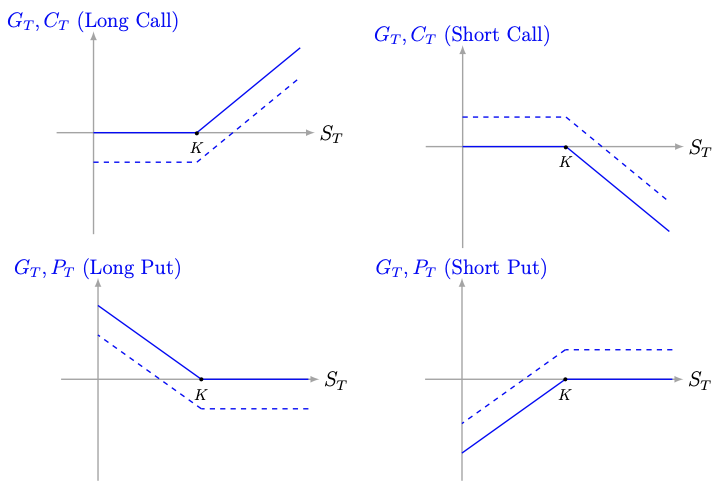
Observe that we have not incorporated the option premium while defining the payoff in the above definition. The gain (or loss) of an option comprises the payoff in addition to the future value of the premium.

Let \(X\) be the premium paid for an option contract, and \(r\) be the prevailing interest rate continuously compounded. Then the gain (or loss) in a call option is defined as

\[ G_T = \left\{\begin{array}{rl} C_T - Xe^{rT},&\text{for long call}\\ Xe^{rT}-C_T,&\text{for short call}\\ \end{array}\right. \]

Similarly, we can define the gain (or loss) in a put option. Illustrations of the gain (depicted by dashed lines) along with the payoff (represented by solid lines) in four possible scenarios are depicted in the following figures.

Gain (dashed lines) and Payoff (solid lines) graphs.

Problem:

An investor buys a 14900-strike put on Nifty when the Nifty is trading in the spot market at 14875 points. The premium for the put is ₹ 27. Assume that the lot size is 100 units and the expiration is 91 days. Considering the prevailing interest rate as 6%, calculate the investor’s gain if the index declines by 75 points from the strike price at expiration. \(~\)

Answer: 4759.31

Hint:

Since the interest rate scheme is not specified, one has to take it as continuous compounding. Also, consider 365 days a year. Note that if the interest rate itself is not given, then take it as zero.

Problem:

Consider a European call option with a 90-strike and 6 months expiration. Given that the underlying stock takes the price ₹ 87, ₹ 92, or ₹ 97 with probability 1/3 each on the expiration date. If the option is bought for ₹ 8 and the prevailing interest rate is 9% continuously compounded, then find the expected gain (or loss) for the long call. \(~\)

Answer: \(-5.3682\)

Remark:

Let us give the formula for the gain in an option using the discrete compounding scheme with frequency \(m\).

The future value of the premium \(X\) at time \(T\) with discrete compounding scheme with frequency \(m\) is given by

\[ \text{FV}(X) = X\left(1+\frac{r}{m}\right)^{mT}. \]

Therefore, the required gain is given by

\[ G_T = \left\{\begin{array}{rl} C_T - X\left(1+\dfrac{r}{m}\right)^{mT},&\text{for long call}\\ X\left(1+\dfrac{r}{m}\right)^{mT}-C_T,&\text{for short call}\\ P_T - X\left(1+\dfrac{r}{m}\right)^{mT},&\text{for long put}\\ X\left(1+\dfrac{r}{m}\right)^{mT}-P_T,&\text{for short put}. \end{array}\right. \]

Time Value in an Option Price

One may argue for considering the intrinsic value of an option as the price of the option. However, the option price is positive at any time \(t\in [0,T)\), whereas the option value, can be zero if the option is out-of-the-money. This shows that an option price includes more than just the intrinsic value.

The option price can be decomposed into (at least) two parts, namely, the intrinsic value and the time value, and is written as Option Price = Intrinsic Value + Time Value. We use the notations \(C^e(t)\) (or \(C^e_t\)) and \(C^a(t)\) (or \(C^a_t\)), \(t\in [0,T]\), to represent European and American call option prices, respectively, and similar notations for other cases.

From the above decomposition, the time value can be written as

\begin{eqnarray} \text{TV}(t)&=& \left\{\begin{array}{ll} C^e(t) - \max\big(0,S(t)-K\big),&\text{for European call}\\ P^e(t) - \max\big(0,K-S(t)\big),&\text{for European put}\\ C^a(t) - \max\big(0,S(t)-K\big),&\text{for American call}\\ P^a(t) - \max\big(0,K-S(t)\big),&\text{for American put}. \end{array}\right. \end{eqnarray}

(4.1)

Option data of a stock as of January 1-st, 2021, for various expirations when the spot price of the stock was ₹ 1260.45 per share.

Example:

Consider a stock on 1\(^{\rm st}\) January 2021 (taken as \(t=0\)) which was trading at ₹ 1260.45 per share. The above table shows the option price for different expirations and different strike prices.

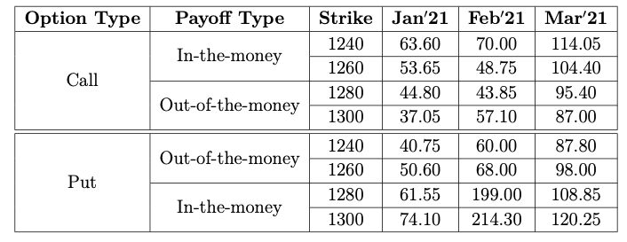
Our interest is to obtain the time value of all the options at \(t=0\) for all the data shown in this table.

Let us take the 1240-strike call option with Jan\(^\prime\)21 expiration, where the option price was \(C^a(0) = 63.6\) and the intrinsic value of the option was

\[ \max\big(0,S(0)-K\big) = \max\big(0,1260.45-1240\big) = 20.45. \]

Therefore, the time value of the option is

\[ \text{TV}^{a}_c(0) = 63.6 - 20.45 = 43.15. \]

The same 1240-strike put option was out-of-the-money and therefore, the intrinsic value is given by

\[ \max\big(0,K-S(t)\big) = \max\big(0,1240-1260.45\big) = 0. \]

Hence, the time value of the option as on 1\(^{\rm st}\) January is

\[ \text{TV}^{a}_p(0) = 40.75. \]

Similarly, we can find the time value for other strike prices and for other expirations.

Premium Bounds and Arbitrage Opportunities

The primary focus of options theory is to determine an appropriate price (premium) for a given option. As we progress into the theory, we will see that this is a difficult task. However, obtaining bounds for the price of an option in a no-arbitrage market is relatively straightforward. Throughout this section, we assume that the market allows short selling and that lending and borrowing occur at the same prevailing interest rate \(r\), with continuous compounding.

European Options

Let us first explore the simplest case of a European option, where the underlying stock does not pay dividends during the option period.

Theorem:

[European Call on Non-Dividend-Paying Stock]

Consider a European call option with

\(K\)-strike;
period \([0,T]\); and
\(t\in [0,T]\) is the present time with premium \(C^e_t\),

where the underlying stock with spot price \(S_t\) pays no dividend during the option period. If the market does not allow arbitrage, then

\[ \max\big(0,S_t - Ke^{-r(T-t)}\big) \le C^e_t \le S_t. \]

where \(r\) is the prevailing annual interest rate continuously compounded.

Proof:

Without loss of generality, we take \(t=0\) and prove the estimate

\[ \max\big(0,S_0 - Ke^{-rT}\big) \le C^e_0 \le S_0. \]

Upper bound: First, let us prove the upper bound.

Assume the contrary that there is a \(K\)-strike call option with premium \(C^e_0> S_0.\) Then, construct a portfolio using the following trades:

short \(K\)-strike call option;
buy the stock in the spot market;
invest \(C^e_0-S_0\) in a risk-free interest rate instrument up to the expiration date of the call option.

The portfolio is given by

\[ \Pi_1 = (\phi,\theta,c);~~\phi=1, \theta=1, c=-1. \]

Here, we assumed that one unit of the risk-free instrument costs \(C^e_0-S_0\) (one may simply assume the risk-free instrument as the savings bank account). The value of the portfolio at \(t=0\) is

\[ V(\Pi_1)(0) = 1\times(C^e_0 - S_0) +1 \times S_0 + (-1)\times C^e_0 = 0. \]

At time \(t=T\), the value of the portfolio \(\Pi_1\) is given by

\[ V(\Pi_1)(T) = (C^e_0 - S_0)e^{rT} + \min\big\{K, S_T\big\}. \]

Since \(K>0\), \(S_T>0\), and by our assumption \(C^e_0>S_0\), we see that \(V(\Pi_1)(T)>0\) and this happens with probability 1.

This shows that \(\Pi_1\) is an arbitrage portfolio. This contradicts the no-arbitrage market assumption.

Lower bound: Let us now prove the lower bound.

It is clear that \(C^e_0\ge 0\). Therefore, we assume that \(S_0 - Ke^{-rT}>0\) and prove that \(S_0 - Ke^{-rT}\le C^e_0\).

Assume the contrary \(S_0 - Ke^{-rT} > C^e_0.\)

Then, we construct a portfolio by making the following trades:

short a stock in the spot market at the price of \(S_0\) per share;
buy one \(K\)-strike call option by paying the premium \(C^e_0\); and
invest \(S_0-C^e_0\) in a risk-free interest rate instrument up to the expiration date of the call option.

The portfolio is given by

\[ \Pi_1 =(\phi,\theta,c);~~\phi=1, \theta=-1, c=1, \]

where we have assumed that one unit of the risk-free asset is \(S_0-C^e_0\). The value of the portfolio at \(t=0\) is

\[ V(\Pi_1)(0) = 1\times(S_0 - C^e_0) + (-1) \times S_0 + 1\times C^e_0 = 0. \]

At time \(t=T\), make the following trades:

close the risk-free investment;
if \(S_T>K\), then exercise the call option;\\ otherwise, buy one stock at the spot market; and
close the short position at the spot market.

The payoff of \(\Pi_1\) is

\[ V(\Pi_1)(T) = (S_0-C^e_0)e^{rT} - \min\big\{K, S_T\big\}. \]

By our assumption, we get (how?)

\[ V(\Pi_1)(T) >0 \]

with probability 1. Thus, \(\Pi_1\) is an arbitrage portfolio.

Theorem:

[European Put on Non-Dividend-Paying Stock]

Consider the European put option

\(K\)-strike;
period \([0,T]\);
\(t\in [0,T]\) is the present time with premium \(P^e_t\),

where the underlying stock with spot price \(S_t\) pays no dividend during the option period. If the market does not allow arbitrage, then

\[ \max\big(0,Ke^{-r(T-t)}-S_t\big) \le P^e_t \le Ke^{-r(T-t)}, \]

where \(r\) is the prevailing annual interest rate continuously compounded.

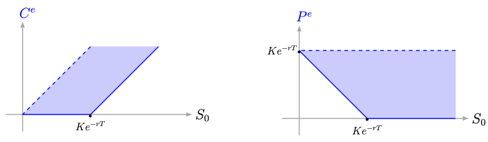
Proof of this theorem is left as an exercise.

The bounds obtained in the above theorem are graphically illustrated in the figure below.

An illustration of the bounds for European call (left) and put (right) options for no-dividend-paying stocks.

Example:

[A real-time illustration]

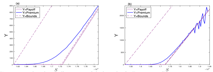
Let us illustrate the bounds proved in Theorem «Click Here» using real-time data. To this end, we have obtained the option chain data for NIFTY with an expiration date of February 24, 2022, from the NSE website

https://www.nseindia.com/option-chain

on February 18, 2022, after the market closed. On that day, NIFTY closed at approximately \(17,276\) points. The last traded price (LTP) of the call options with various strike prices were extracted from the downloaded option chain table. These premiums are depicted in the figure below by a solid blue line, where the roles of the strike price and spot price are interchanged. The dashed lines represent the corresponding bounds obtained from Theorem «Click Here» , while the payoff graph is illustrated by a solid line.

The lower bound is calculated using \(K=17250\) and \(r=0.0675\), which is approximately the 10-year government bond yield as of the last week of February 2022. In the (a) part of the following figure, a zoomed view around \(K\) is provided, representing the nearly at-the-money options.

From this figure, it is evident that there are no arbitrage opportunities according to the considered interest rate \(r\). This can be attributed to the substantial liquidity present in these options. However, as we move away from the at-the-money option, liquidity diminishes, and sometimes visible arbitrage opportunities emerge, particularly at the market's closing time, due to speculators. This phenomenon is clearly observed in the (b)-part of the following figure around strikes greater than 18700, which correspond to far in-the-money options. It is worth noting that at the next day's market opening, such arbitrage gaps either cease to exist or are swiftly filled by arbitrageurs.

A real-time illustration of the bounds of a European call option premium proved in Theorem «Click Here» . Details are in Example «Click Here» .

Problem:

[European Options on Dividend-Paying Stock]

Consider the European (call or put) options with

\(K\)-strike;
period \([0,T]\);
premium \(C^e_t\) for call and \(P^e_t\) for put,

where \(t\in [0,T)\) is the present time with the spot price of the underlying asset \(S_t\) that pays dividend \(D\) at some known time \(t_1\in (t,T)\). If the market does not allow arbitrage, then show that

\begin{eqnarray} \begin{array}{cl} \max\big(0,S_t - De^{-r(t_1-t)} - Ke^{-r(T-t)}\big) \le C^e_t \le S_t - De^{-r(t_1-t)},&\text{ for call option;}\\ \max\big(0,Ke^{-r(T-t)} -S_t+ De^{-r(t_1-t)}\big) \le P^e_t \le Ke^{-r(T-t)},&\text{ for put option,} \end{array} \end{eqnarray}

(4.2)

where \(r\) is the prevailing annual interest rate continuously compounded.

Project:

Write a Python code that takes the following inputs:

The name of the CSV file containing an option chain for NIFTY (download the CSV file from the website provided in Example «Click Here» );
The spot market value of NIFTY corresponding to the option chain given in the CSV file;
The prevailing interest rate;
The expiration time \(T\).

Furthermore, the Python code should perform the following:

Read the CSV file;
Identify all arbitrage opportunities in the option chain based on the estimates provided in Theorem «Click Here» and Theorem «Click Here» ;
Display the identified opportunities along with the arbitrage gain.

American Options

We now turn our attention to obtaining bounds for an American option premium.

It is important to note that American options offer more flexibility than European options. Consequently, one might expect the premium of an American option to be higher than that of a European option with the same parameters.

Problem:

Consider two options (either both call or both put):

\(K\)-strike, call option;
option period is \([0,T]\); and
premium of \(X^e\) for the European option and \(X^a\) for the American option.

If the underlying stock does not pay dividend during the option period, the market does not allow arbitrage, and the prevailing interest rate is \(r > 0\), then prove that

\[ X^e \le X^a. \]

Hint:

Take a long position in one contract (European or American, as appropriate) and take a short position in the other contract. Hold the positions until expiration. At expiration, we must settle both options simultaneously. It is important to note that we must justify arbitrage. For this purpose, the settlement should be viewed as follows:

Borrow the amount \(S_T\);
Settle the contract where we have to buy the asset;
Supply the asset in the other contract and receive \(S_T\);
Repay the borrowed money.

This way, we do not need to pay any interest for the borrowing as the borrowing and repayment occur immediately.

Note:

In the above result, the absence of a specified time component indicates that the result remains consistent irrespective of the time variable.

In particular, for call options, we always have \(C^e = C^a\) when the underlying asset is a non-dividend-paying stock.

Problem:

Consider two call options with

\(K\)-strike;
option period \([0,T]\); and
premium of \(C^e\) for the European option and \(C^a\) for the American option.

If the underlying stock does not pay dividend during the option period, the market does not allow arbitrage, and the prevailing interest rate is \(r > 0\), then prove that

\[ C^e = C^a. \]

Note:

The above result does not hold if the underlying stock pays dividends sometime during the option period. Also, the result does not hold for American put options.

The following theorem is a direct consequence of Theorem «Click Here» and Problem «Click Here»

Theorem:

[American Call on Non-Dividend-Paying Stock]

Consider an American call option with

\(K\)-strike;
period \([0,T]\); and
\(t\in [0,T)\) is the present time with premium \(C^a_t\),

where the underlying stock with spot price \(S_t\) pays no dividend during the option period. If the market does not allow arbitrage, then

\[ \max\big(0,S_t - Ke^{-r(T-t)}\big) \le C^a_t \le S_t, \]

where \(r\) is the prevailing annual interest rate continuously compounded.

As noted above, in the case of put options, we have \(P^e \leq P^a\) even if the underlying stock does not pay a dividend during the option period. Therefore, it is crucial to investigate the bounds for American put options. As usual, we begin by considering non-dividend paying stocks as the underlying asset.

Problem:

[American Put on Non-Dividend-Paying Stock]

Consider the American put option with

\(K\)-strike;
period \([0,T]\);
\(t\in [0,T)\) is the present time with premium \(P^a_t\),

where the underlying stock has a spot price of \(S_t\) per unit and pays no dividend during the option period. If the market does not allow arbitrage, then show that

\[ \max\big(0,K-S_t\big) \le P^a_t \le K. \]

We can obtain the bounds for American options for dividend paying stocks by combining all the results stated so far.

Problem:

[American Options on Dividend-Paying Stock]

Consider the American (call or put) option with

\(K\)-strike;
period \([0,T]\);
premium \(C^a_t\) for call and \(P^a_t\) for put,

where the stock pays dividend \(D\) at some known time \(t_1\in (t,T)\) and \(t\in [0,t_1)\) is the present time with the spot price \(S_t\). If the market does not allow arbitrage and the exercise time \(\tau > t_1\), then show that

\begin{eqnarray} \begin{array}{cl} \max\big(0,S_t - De^{-r(t_1-t)} - Ke^{-r(T-t)}, S_t-K\big) \le C^a_t \le S_t - De^{-r(t_1-t)},&\hspace{-0.1in}\text{for call option;}\\ \max\big(0,Ke^{-r(T-t)}+ De^{-r(t_1-t)} -S_t, K-S_t\big) \le P^a_t \le K,&\hspace{-0.1in}\text{for put option,} \end{array} \end{eqnarray}

(4.3)

where \(r\) is the prevailing annual interest rate continuously compounded.

Put-Call Parity Estimates

So far, we have obtained the bounds for call and put options. Now, we will discuss the relationship between call and put options in both European and American types.

Let us begin by examining European options and establishing the relationship.

Theorem:

[Put-Call Parity for European Options]

Consider two European options, one call and one put with

\(K\)-strike;
period \([0,T]\); and
the premium \(C^e_t\) for the call option and the premium \(P^e_t\) for the put option are at the present time \(t\in [0,T)\).

Let the underlying stock have the spot price of \(S_t\) pays no dividends during the option period. If the market does not allow arbitrage, then

\[ C^e_t - P^e_t = S_t - Ke^{-r(T-t)}, \]

where \(r\) is the prevailing annual interest rate continuously compounded.

Proof:

We prove the theorem for \(t=0\).

Case 1: Assume the contrary that \(C^e_0 - P^e_0 > S_0 - Ke^{-rT}.\)

Let us construct the portfolio \(\Pi_1\) using the following trades:

buy a share at the spot market for \(S_0\) per share;
take a long position in one put option;
write one call option; and
invest (or borrow if negative) the sum \(C^e_0-P^e_0-S_0\) in a risk-free interest rate investment.

It can be seen that \(V(\Pi_1)(0) = 0.\) At time \(t=T\), we have

\[ V(\Pi_1)(T) = (C^e_0-P^e_0-S_0)e^{rT} + K > 0, \]

by our assumption. Complete the proof.

Case 2: Assume the contrary that \(C^e_0 - P^e_0 < S_0 - Ke^{-rT}.\)

Let us construct the portfolio \(\Pi_1\) using the following trades:

short a share at the spot market for \(S_0\) per share;
write one put option;
go long in one call option; and
invest (or borrow if negative) the sum \(S_0-C^e_0+P_0^e\) in a risk-free interest rate investment.

Complete the proof.

We now obtain the put-call parity for American options.

Theorem:

[Put-Call Parity for American Options]

Consider two American options, one call and one put with

\(K\)-strike;
period \([0,T]\); and
premium \(C^a_t\) for the call option and \(P^a_t\) for the put option are at the present time \(t\in [0,T).\)

Let the underlying stock have the spot price of \(S_t\) pays no dividends during the option period. If the market does not allow arbitrage, then

\[ S_t-K \le C^a_t - P^a_t \le S_t - Ke^{-r(T-t)}, \]

where \(r\) is the prevailing annual interest rate continuously compounded.

Proof:

The upper bound is a direct consequence of Theorem «Click Here» and Theorem «Click Here» . However, we give the arbitrage portfolio argument.

We prove the result for \(t=0\).

Let us first consider the upper bound.

Assume the contrary that \(C^a_0-P^a_0-S_0+Ke^{-rT} > 0\).

Construct the portfolio \(\Pi_1\) with the following trades:

write one call option and get the premium \(C^a_0\);
buy one put option by paying the premium \(P^a_0\);
buy one share by paying \(S_0\); and
invest (borrow if negative) the remaining \(C^a_0-P^a_0-S_0\) in a risk-free interest rate investment.

The initial value of \(\Pi_1\) is given by \(V(\Pi_1)(0) = 0.\)

Let \(t=\tau\in [0,T]\) be the exercise time of the short call option. The payoff of \(\Pi_1\) at \(t=\tau\) is

\[ V(\Pi_1)(\tau) = (C^a_0-P^a_0-S_0)e^{r\tau} + K. \]

Using our assumption, we can see that \(V(\Pi_1)(\tau) > 0\) (how?). From the above inequality, we can see that, although \(\tau\) and \(S_\tau\) are random, finally, the required positivity does not depend on these variables. Thus, the positivity of the portfolio happens with probability 1, and therefore \(\Pi_1\) is an arbitrage portfolio.

Let us now consider the lower bound.

Assume the contrary that \(C^a_0 - P^a_0 - S_0 + K < 0\).

Construct the portfolio \(\Pi_1\) with the following trades:

write one put option and get the premium \(P^a_0\);
buy one call option by paying the premium \(C^a_0\);
short one share and get \(S_0\); and
invest (borrow if negative) the remaining \(P_0^a-C_0^a+S_0\) in a risk-free interest rate investment.

The initial value of \(\Pi_1\) is given by \(V(\Pi_1)(0) = 0.\)

Let \(t=\tau\in [0,T]\) be the exercise time of the short put option. The payoff of \(\Pi_1\) at \(t=\tau\) is

\[ V(\Pi_1)(\tau) = (P^a_0-C^a_0+S_0)e^{r\tau} - K. \]

From our assumption, we see that \(V(\Pi_1)(\tau)>0\) (how?). Complete the arbitrage arguement.

Premium Valuation

So far, we have studied some important estimates of call and put options having the same strike price. In this subsection, we study some basic properties of options prices depending on their strike prices. Let us include the strike price into the notation of option prices.

Remark:

For a given expiration \(T\), we use the following notations:

For any \(t\in [0,T]\) and for a positive real number \(K\),

\(C^e(t,K)\) or \(C^e_t(K)\) denotes the European call option price (or premium) at time \(t\) whose strike price is \(K\). For an American call option, we use the notation \(C^a(t,K)\) or \(C^a_t(K)\).
\(P^e(t,K)\) or \(P^e_t(K)\) denotes the European put option price (or premium) at time \(t\) whose strike price is \(K\). For an American put option, we use the notation \(P^a(t, K)\) or \(P^a_t(K)\).

Theorem:

[Dependency on strike price: European]

If the underlying stock does not pay a dividend during the option period and the market does not allow arbitrage, then

\begin{eqnarray} 0\le C^e_t(K_1 ) - C^e_t(K_2 ) \le e^{-r(T-t)}\big(K_2 - K_1\big),\\ 0\le P^e_t(K_2 ) - P^e_t(K_1 ) \le e^{-r(T-t)}\big(K_2 - K_1\big), \end{eqnarray}

(4.4)

for any \(0\le K_1 \le K_2,\) where \(r\) is the prevailing interest rate continuously compounded, all the options have the same period \([0,T]\) and \(t\in [0,T)\) is the present time.

Proof:

\(~\) We prove the theorem with \(t=0\).

Let us first consider the lower bound.

Lower bound for call options:
Assume the contrary that \(C^e_0(K_1 ) < C^e_0(K_2 ).\)
Construct a portfolio \(\Pi_1\) using the following trades:
1. write the \(K_2\)-strike call option;
2. buy the \(K_1\)-strike call option; and
3. invest \(C^e_0(K_2 ) - C^e_0(K_1 )\) in a risk-free interest rate investment.
The initial value of \(\Pi_1\) is \(V(\Pi_1)(0) = 0.\)
At time \(t=T\), the value of \(\Pi_1\) is
\[ V(\Pi_1)(T) = (C^e_0(K_2 ) - C^e_0(K_1 )) e^{rT} + x_0, \]
where
\[ x_0 = \left\{\begin{array}{ll} K_2-K_1, &\text{if } K_2 < S_T\\ S_T-K_1,&\text{if } K_1 < S_T\le K_2\\ 0,&\text{if } S_T \le K_1. \end{array}\right. \]
Since \(K_1\le K_2\) and by our assumption, we see that \(V(\Pi_1)(T) > 0\), leading to a contradiction to the no-arbitrage principle.
Lower bound for put option: Left as an exercise.
Upper bound for both: By put-call parity result from Theorem «Click Here» , we have
\begin{eqnarray} C^e_0(K_1 ) - P_0^e(K_1 ) = S_0 - K_1e^{-rT},\\ C^e_0(K_2 ) - P_0^e(K_2 ) = S_0 - K_2e^{-rT}. \end{eqnarray}
(4.5)
Subtracting, we get
\[ \big(C^e_0(K_1 ) - C^e_0(K_2 )\big) + \big(P^e_0(K_2 ) - P^e_0(K_1 )\big) = (K_2 - K_1)e^{-rT}. \]
Since both the terms in the brackets on the left-hand side are nonnegative as per the lower bounds, we see that each one is less than or equal to the right-hand side.

Problem:

Prove the upper bounds in the above theorem using arbitrage arguments.

Remark:

From the lower bound, we see that the call option price is a non-increasing function of \(K\) and the put option price is a non-decreasing function of \(K\). Also, we see from the upper bound that both the call option and the put option prices are Lipschitz functions.

In the next theorem, we show that \(C^e\) and \(P^e\) are convex functions of \(K\), a characteristic often observed in the market. However, the mathematical proof requires the assumption that the market allows trading fractional units.

Theorem:

[Convexity property: European]

Assume that the market does not allow arbitrage, permits fractional unit trades, and allows short selling. For any \(\alpha\in [0,1]\) and for any positive real numbers \(K_1\) and \(K_2\), we have

\begin{eqnarray} C^e\big(\alpha K_1 + (1-\alpha)K_2 \big) \le \alpha C^e(K_1 ) + (1-\alpha)C^e(K_2 ),\\ P^e\big(\alpha K_1 + (1-\alpha)K_2 \big) \le \alpha P^e(K_1 ) + (1-\alpha)P^e(K_2 ), \end{eqnarray}

(4.6)

where all the options have the same expiration.

Proof:

Let us use the notation

\[ K = \alpha K_1 + (1-\alpha)K_2. \]

Call Option: Assume the contrary that

\[ C^e\big(K \big)> \alpha C^e(K_1 ) + (1-\alpha)C^e(K_2 ). \]

Construct a portfolio \(\Pi_1\) using the following strategies:

write the \(K\)-strike call option;
buy \(\alpha\) units of \(K_1\)-strike call options;
buy \(1-\alpha\) units of \(K_2\)-strike call options; and
invest \(C^e\big(K \big)-\big(\alpha C^e(K_1 ) + (1-\alpha)C^e(K_2 )\big)\) in a risk-free interest rate instrument.

We have \(V(\Pi_1)(0) = 0\), and at time \(t=T\), we have

\begin{eqnarray} V(\Pi_1)(T) &=& \Big(C^e\big(K \big)-\big(\alpha C^e(K_1 ) + (1-\alpha)C^e(K_2 )\big)\Big)e^{rT} + x_0, \end{eqnarray}

(4.7)

where

\[ x_0 = \left\{\begin{array}{ll} \left\{\begin{array}{ll} \alpha (S_T -K_1),&\text{if } K_1 < S_T \text{ and } K_2\ge S_T\\ (1-\alpha) (S_T -K_2),&\text{if } K_1\ge S_T \text{ and } K_2 < S_T\\ 0,&\text{if } K_1\ge S_T \text{ and } K_2\ge S_T\\ \end{array}\right. , &\text{if } K\ge S_T,\\ K - \left\{\begin{array}{ll} \alpha K_1 + (1-\alpha)K_2,&\text{if } K_1 < S_T \text{ and } K_2 < S_T\\ \alpha K_1 + (1-\alpha)S_T,&\text{if } K_1 < S_T \text{ and } K_2 \ge S_T\\ \alpha S_T + (1-\alpha)K_2,&\text{if } K_1 \ge S_T \text{ and } K_2 < S_T \end{array}\right. ,& \text{if } K < S_T. \end{array}\right. \]

It can be proved that \(x_0\ge 0\).

Put Option: Convexity of the put option price can be proved in two ways,

by constructing an arbitrage portfolio; and
using convexity of call option price and the put-call parity result in Theorem «Click Here» .

We leave the first method as an exercise and prove the result using the second method.

We prove the result for \(t=0\).

From Theorem «Click Here» , we have

\begin{eqnarray} C^e_0(K ) - P^e_0(K ) &=& S_0 - Ke^{-rT} \end{eqnarray}

(4.8)

This implies

\begin{eqnarray} P^e_0(K ) &\le &\alpha C^e_0(K_1 ) + (1-\alpha)C^e_0(K_2 )+ Ke^{-rT} - S_0\\ &=&\alpha \Big(C^e_0(K_1 ) +K_1e^{-rT}-S_0\Big) + (1-\alpha) \Big(C^e_0(K_2 ) +K_2e^{-rT}-S_0\Big) \end{eqnarray}

(4.9)

Again using Theorem «Click Here» , we get the desired result.

We now state the equivalent theorems in the case of American options. The proofs are left as exercises.

Problem:

[Dependency on strike price: American]

If the underlying stock does not pay a dividend during the option period and the market does not allow arbitrage, then show that

\begin{eqnarray} 0\le C^a_t(K_1 ) - C^a_t(K_2 ) \le e^{-r(T-t)}\big(K_2 - K_1\big),\\ 0\le P^a_t(K_2 ) - P^a_t(K_1 ) \le K_2 - K_1, \end{eqnarray}

(4.10)

for any \(0\le K_1 \le K_2,\) where \(r\) is the prevailing interest rate continuously compounded, all the options have the same period \([0,T]\), and \(t\in [0,T)\) is the present time.

Problem:

[Convexity property: American]

For any \(\alpha\in [0,1]\) and for any positive real numbers \(K_1\) and \(K_2\), show that

\begin{eqnarray} C^a\big(\alpha K_1 + (1-\alpha)K_2 \big) \le \alpha C^a(K_1 ) + (1-\alpha)C^a(K_2 ),\\ P^a\big(\alpha K_1 + (1-\alpha)K_2 \big) \le \alpha P^a(K_1 ) + (1-\alpha)P^a(K_2 ), \end{eqnarray}

(4.11)

where all the options have the same period \([0,T]\), and the market does not allow arbitrage.